Algorithm description for six-degree-of-freedom pose estimation using GPS and IMU.
For detailed mathematical derivations (Jacobians, prediction/update steps), see MOKUKU-INS/6dof.
1. Algorithm Overview
An Error State Iterated Kalman Filter (ESIKF) is used for tightly-coupled fusion of IMU and GNSS to estimate 6DoF pose (position + orientation). The filter operates on manifolds.
2. State Variables and Coordinate Frames
2.1 State Vector
| State Variable | Dimension | Description |
|---|---|---|
pos |
3 | Position of IMU body frame origin in local UTM coordinates |
rot |
3 (SO3) | Rotation of IMU body frame with respect to world frame |
vel |
3 | IMU velocity in world frame |
bg |
3 | Gyroscope bias |
ba |
3 | Accelerometer bias |
gnss_extrinsic |
3 | Translation of GNSS antenna in IMU body frame |
gnss_extrinsic_rot |
3 (SO3) | Rotation extrinsic from GNSS to IMU |
car_extrinsic_rot |
3 (SO3) | Rotation extrinsic from IMU to vehicle body |
grav |
2 (S2) | Gravity direction (normalized) |
2.2 Coordinate Frame Conventions
- World frame: Local UTM coordinate system, Z-axis up
- Body frame: IMU coordinate system
- GNSS position:
pos + rot * gnss_extrinsicgives antenna position in world frame
3. Prediction Model (IMU)
The IMU serves as the prediction step; standard INS propagation equations are used:
ẋ = f(x, u)
Where:
- Position:
ṗ = v - Rotation:
ṙ = ω - bg(angular velocity integration) - Velocity:
v̇ = R(a - ba) + g(acceleration transformed to world frame plus gravity)
R is the rotation matrix from body to world frame; ω and a are gyroscope and accelerometer measurements.
4. Measurement Model (GNSS)
4.1 Position Measurement
- GNSS provides LLA coordinates; convert to UTM and subtract
originto obtain local position - Observation covariance is set according to
solve_status - 2D scenario: Set elevation component to zero
measurement(2) = 0to enforce planar motion (for trajectory visualization only) - 3D scenario: Use full 3D position measurement
4.2 Heading Measurement
- Use GNSS heading (yaw angle) and optionally pitch
- Heading only:
rotation_heading = AngleAxis(heading, Z) - Heading + pitch:
rotation_heading = AngleAxis(heading, Z) * AngleAxis(pitch, Y) - Measurement validity is determined by thresholds such as
hdgstddev
4.3 Velocity-Related Measurements
- Use GNSS horizontal speed for zero-velocity detection and initialization
- Forward velocity constraint: Constrain lateral and vertical velocity to near zero by using different covariance for each velocity component (e.g.
[1e-6, 1e4, 1e-6]) - Optional: velocity magnitude measurement
‖v‖² = speed²
5. Zero-Velocity Update (ZUPT)
When stationary, apply zero-velocity constraint to suppress drift:
Detection conditions (use example thresholds):
- Filter velocity magnitude < 0.4 m/s
- Linear acceleration magnitude close to gravity (abs(‖a‖ - g) < 0.1)
- Angular velocity magnitude < 0.1 rad/s
- GNSS horizontal speed < 0.4 m/s
When satisfied, use zero-velocity observation v = 0 to update the filter state.
6. Initialization
- Wait for first valid GNSS position and velocity
- Initialize rotation using GNSS heading (and optionally pitch)
- Initialize velocity using GNSS velocity projected into body frame
- Set first GNSS position as
origin; subsequent positions are expressed relative to this origin
7. Output Smoothing
To avoid pose discontinuities from GNSS updates, apply smoothen_offset smoothing:
- Keep “smoothed pose” continuous across GNSS updates
- Control smoothing strength via
smoothen_ratio(smaller = smoother) - Skip smoothing during initialization (e.g. first 5 seconds) for faster convergence
8. Algorithm Flow Overview
                  ┌─────────────┐
                  │  GNSS Input │
                  └──────┬──────┘
                         │
       ┌─────────────────┼─────────────────┐
       │                 │                 │
       ▼                 ▼                 ▼
   ┌──────────┐     ┌──────────┐     ┌──────────┐
   │ Position │     │ Heading  │     │ Velocity │
   │  Measure │     │  Measure │     │  (ZUPT   │
   │          │     │(+Pitch?) │     │  detect) │
   └────┬─────┘     └────┬─────┘     └────┬─────┘
        │                │                │
        └────────────────┼────────────────┘
                         │
                         ▼
              ┌──────────────────────┐
              │   ESIKF Filter       │
              │  ┌────────────────┐  │
              │  │ IMU Predict    │  │
              │  └────────┬───────┘  │
              │           │          │
              │  ┌────────▼───────┐  │
              │  │ GNSS Update    │  │
              │  └────────────────┘  │
              └──────────┬───────────┘
                         │
                         ▼
              ┌──────────────────────┐
              │  6DoF Pose Output    │
              │  (pos, rot, vel)     │
              └──────────────────────┘
9. Estimation Result
Output format
The 6DoF pose is output with the following columns:
| Column | Unit | Description |
|---|---|---|
| timestamp | s | Timestamp in seconds |
| pos_x | m | UTM Easting |
| pos_y | m | UTM Northing |
| pos_z | m | Height |
| qx | - | Quaternion x |
| qy | - | Quaternion y |
| qz | - | Quaternion z |
| qw | - | Quaternion w |
output example:
timestamp,pos_x,pos_y,pos_z,qx,qy,qz,qw
0.0000000000000,746569.2267269332660,2560297.0387227563187,10.1508998986581,0.0123424213859,0.0126907274138,-0.6970915044935,0.7167635903386
0.0062505170000,746569.2267408345360,2560297.0387173718773,10.1508998672053,0.0028215518808,-0.0174815944078,0.9911133379082,0.1318362018662
0.0261357400000,746569.2266839033691,2560297.0387508110143,10.1508983113788,0.0028215518759,-0.0174815944075,0.9911133379079,0.1318362018681
...
Trajectory visualization
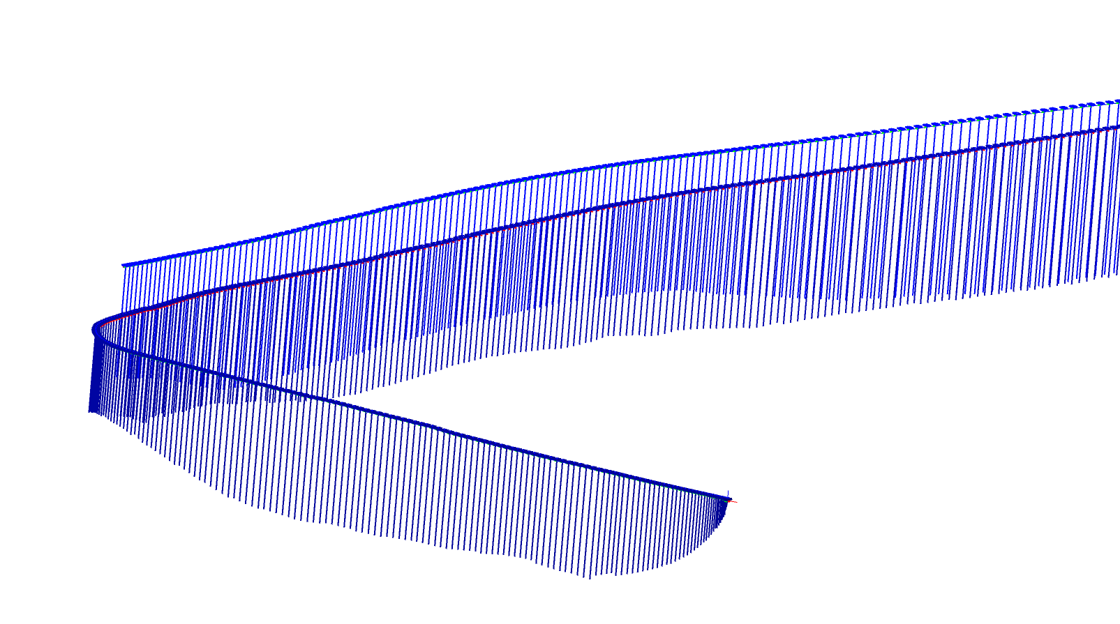
- Bridge scenario: The vertical lines below the trajectory represent velocity magnitude. Both speed and position change smoothly.
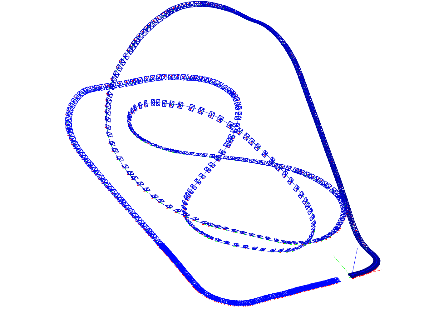
- Roller coaster scenario: The algorithm estimates angle changes during motion well, and position estimation remains smooth.